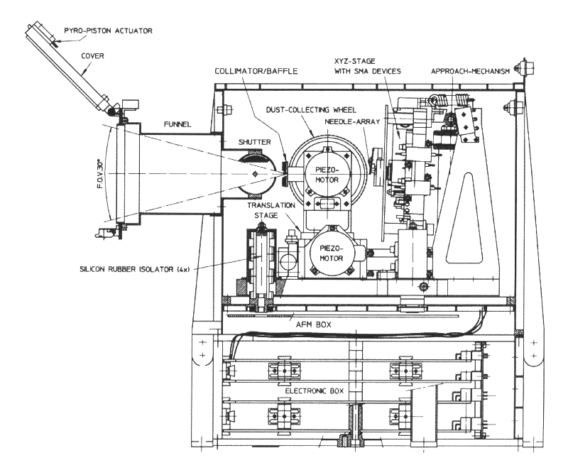
Throughout the 957 hibernation period of Rosetta, MIDAS has been in its “exposure” mode, with a clean target positioned at the funnel and the shutter open – see the diagram below to get an idea of the gemoetry. Although the Solar System is full of dust, we didn’t expect to collect much, if anything; after all MIDAS has only a small opening to let dust in, and a small collector behind it. But we did it anyway. Firstly because… well, why not! With no power available to run the instruments during hibernation, at least this way there was a chance we could do some science. But also as a safety measure – if the shutter were to jam after the cold of hibernation, at least we could still operate the instrument!
In this, our third re-commissioning slot, we want to perform our first real scan since hibernation. This lets us check out the newly upgrade flight software, do a real test of the instrument, and check if perhaps we did collect some dust during hibernation. This test is partially non-interactive (the commands are stored on-board the spacecraft and sent to MIDAS at specific times) and partially interactive. In this latter part we want to test upgrades to our feature recognition algorithm. Since operations on-board Rosetta have to be planned in advance, and an atomic force microscope is usually a “hands on” instrument, we have to bridge this gap with software.
To do this we have scheduled a scan and then let the software examine the image and determine if there are any dust particles present. If so, the on-board software automatically sets up the microscope to look at the most prominent feature in a subsequent scan. In this case we decided on a 160×192 pixel image with a resolution of about 210 nm (one nanometre is one millionth of a metre!), making an image size of about 34×40 µm. The image data will be transmitted to Earth at the end of the non-interactive part of the exercise, along with the features in the image that the software has found. MIDAS will also automatically set up the next scan based on the discovered features.
The MIDAS team will be sitting at ESOC, the ESA control centre in Darmstadt, Germany, waiting for these data to be downloaded. We will then look at the image and compare the features that we would choose to zoom in on with those that the software found. If necessary we will update the coordinates for our zoom image (this is why we need the interactive part!) and upload these to MIDAS.
By the end of this exercise we will have fully tested MIDAS, but we’re not quite finished with the re-commissioning yet! To make good scientific measurements it is always necessary to calibrate equipment and the same is true for MIDAS. To make sure that our scanner (the unit that moves our sharp tips in three dimensions: X, Y and Z) measures a nanometre as a nanometre we carry several on-board calibration targets. By periodically taking images of these targets we can be sure that all of our scientific images can be labelled with real units.
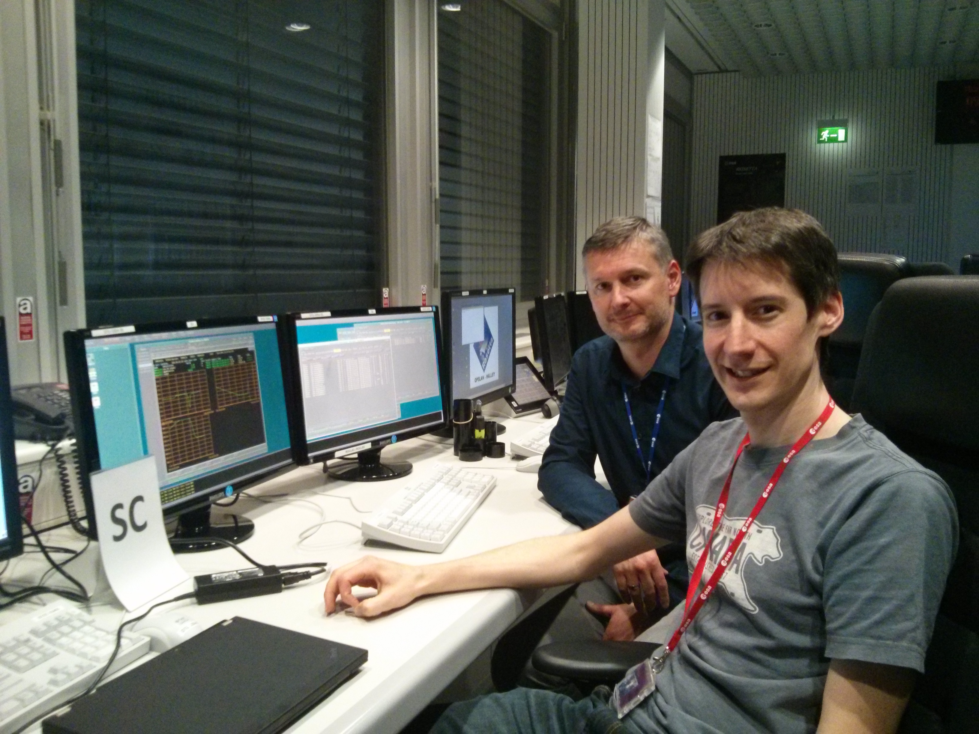
Update 31/03/2014: reporting live from ESA Operations / ESOC
As well as tweeting, I figured I could add some more details more-or-less live here… The MIDAS operations that were running non-interactively completed… but not with all green lights. The commanding of MIDAS is quite complex, and it turns out I had set a parameter incorrectly (my bad!). As a result, we are changing the plan for this evening slightly from the above. Instead of commanding a follow-up zoom in the interactive slot, we will repeat the failed operations from our non-interactive slot – basically we will still image the DSH hibernation target, and still test the zoom function, but not have the chance today to follow-up “live”. That will have to wait for a later opportunity.
Now to the specifics… an AFM running in dynamic mode uses cantilever which is oscillated at close to its resonance frequency. The specific cantilever chosen for the scans tonight has the following resonance curve (taking during our first re-commissioning activity):
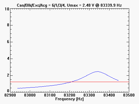
The on-board software then knows where the peak of this curve is, and uses the frequency and amplitude of this peak to control the microscope. To find this resonance peak we command a frequency sweep, characterised by start frequency, a frequency step, and a number of scan blocks. Each block has 256 frequency steps, so with a step of 1 Hz, each block covers 256 Hz. For tonight’s scan we had a start frequency of 82210 Hz, and should have scanned over a range of 2048 Hz, with 8 blocks each with a step size of 1 Hz. This is where my entering 1, instead of 8, caused problems. Instead of scanned only from 82210 Hz + 256 Hz = 82466 Hz. As you can see from the graph above, this is nowhere close to the necessary frequency range. So when we got the data back from Rosetta, the curve looked like:
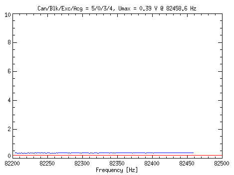
Not quite what we hoped for, but it’s clear why it failed! Fortunately the nature of the subsequent interactive slot means we can actively send the commands to the spacecraft and instrument straight away, and run the test again!
22:30 – now we have live telemetry from MIDAS and are much happier 🙂
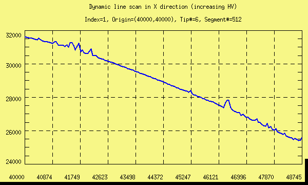
And here is our first line scan! Before rastering across the surface of a sample, we did a simple linear scan to check how things worked. We also requested some diagnostic data during this scan (which we can’t do during a full image scan because it would generate too much data)…